Computed Tomography (CT) Automatic Exposure Controls (AEC) Testing Protocol Using a CelT Phantom
Keolathile Diteko, Rebecca Duguid and Lee Hampson
Keolathile Diteko1*, Rebecca Duguid2 and Lee Hampson2
1International Atomic Energy Agency (IAEA), University of Aberdeen, Aberdeen, Scotland, UK
2Aberdeen Royal Infirmary, University of Aberdeen, Aberdeen, Scotland, UK
- *Corresponding Author:
- Keolathile Diteko
International Atomic Energy Agency (IAEA) Fellow
University of Aberdeen
Aberdeen, Scotland, UK
Tel: 26772301684
E-mail: ditytso@hotmail.com
Received Date: May 18, 2020; Accepted Date: May 29, 2020; Published Date: June 10, 2020
Citation: Diteko K, Duguid R, Hampson L (2020) Computed Tomography (CT) Automatic Exposure Controls (AEC) Testing Protocol Using a CelT Phantom. Insights Med Phys. Vol.5 No.1:4.
Copyright: © 2020 Diteko K, et al. This is an open-access article distributed under the terms of the Creative Commons Attribution License, which permits unrestricted use, distribution, and reproduction in any medium, provided the original author and source are credited.
Abstract
The purpose of this research was to set-up a protocol for using the CeIT elliptical test phantom to test the performance of Automatic Exposure Control (AEC) systems on the CT scanners in use at Aberdeen Royal Infirmary (ARI). These are the GE Lightspeed, GE Optima 6600 and Siemens Somaton Definition in Radiology and the Philips Brilliance in Radiotherapy treatment planning. The variation of image noise and the tube current-time product (mAs) were studied from images obtained from each scanner. Noise was measured using the standard deviation of five selected regions of interest in the images of the phantom obtained from the CT scanners. Normalised percentage noise (noise %) was then calculated to compare how the scanners dealt with image noise with relation to the mAs. The results showed an increase in mAs values (increase in dose) with the phantom and regulation of the noise leading to acquisition of quality images from all three scanners. Offcentering, using the AP scout increased the dose to the phantom when the patient table was above the isocenter and reduced the dose to the phantom when the table was below the isocenter. This shows the importance of patient centering for effective AEC system ’ s dose regulation. Different SPRs also affected the operations of the AEC systems differently, with PA giving more dose followed by LAT and AP in the GE and Philips scanners which were studied on this aspect. The Philips D-DOM modulation kept almost constant dose across the scanning process regardless of the phantom size, hence D-DOM should be used with care. CeLT phantom was useful in studying dose regulation by different AEC systems, hence it is useful in quality control (QC) tests of AEC systems on CT scanners as a testing protocol was formulated from this study.
Keywords
Automatic Exposure Control (AEC); Computed Tomography (CT), Image Noise; Attenuation Coefficient; CT Numbers; Stochastic; Deterministic; Radiation exposure; CeLT Phantom; Patient dose; mAs; Hounsfield units
Introduction
The increased worldwide demand for computed tomography (CT) scans to provide quality images and faster scans for patient care and management has led to the introduction of multidetector technology of CT scanners that provide faster scan times, longer scan ranges and higher resolution for better image quality. The demand for CT scans has therefore resulted in the use of more ionising radiation for diagnostic and radiotherapy treatment planning purposes. Radiation dose should be as low as reasonably achievable (ALARA) and the benefits of the radiation procedure should outweigh the risks. The International Commission on Radiation Protection (ICRP) requires diagnostic reference levels (DRLs) to be established to identify abnormally high dose levels by setting an upper threshold, which standard dose levels are not expected to exceed when good practice is applied [1]. The radiation dose received from a CT scan varies from person to person as it depends on the individual’s size, the type of CT procedure used, as well as the type of the CT scanner used. Various dose reduction techniques have been studied to cater for adverse radiation effects, while maintaining the diagnostic utility of the acquired images. Automatic exposure control, minimising scanning times and optimization of system parameters are some of the techniques used in dose reduction to patients [2-4].
Computed Tomography (CT)
Computed tomography (CT) also known as computed axial tomography (CAT) is a non-invasive medical procedure that uses specialized X-ray equipment to produce images of the body. Tomography refers to the ability to view an anatomic section or slice through the body. Cross-sectional images represent a slice of the patient/object being imaged [3,5]. CT scanners make measurements of X-rays attenuation (reduction of X-ray intensity as it passes through matter) through a finite-thickness cross section of the body. The image is represented by a matrix, which is a two-dimensional (2D) array of numbers arranged in rows and columns. The value of the image is represented by each number at that location. Each number in the image matrix represents a 3D volume element (voxel) in the object, while the voxel is represented in the image as a 2D picture element (pixel). The acquired data is reconstructed to form a digital image of the cross section with each pixel in the image representing a measurement of the mean attenuation of a voxel that extends through the thickness of the section.
X-ray attenuation and CT numbers
The attenuation of the radiation through a material of thickness, Δx, can be expressed using equation 1 below:
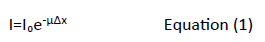
Where I is the X-ray intensity measured with the material in the X-ray beam path, I0 is the X-ray intensity measured without the material in the X-ray beam path, and μ being the attenuation coefficient of the material. The attenuation coefficient reflects the degree of X-ray intensity reduction by a material. The radiation therefore passes through a stack of voxels (as it is attenuated at each voxel) before it is detected. Each attenuation measurement adds up to the sum of attenuation along the ray path through the material. The transmitted intensity is then given by equation 2:
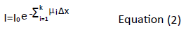
Where

The formula can further be expressed as the natural logarithm (ln):
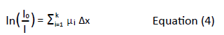
The average attenuation coefficient values (μ) for each voxel in the cross section are derived by an image reconstruction process. The voxel’s average attenuation is found to increase with the density and the atomic number of tissues and it declines with increasing X-ray energy.
The final step of image reconstruction involves scaling of the individual attenuation values to more convenient whole numbers, CT numbers (CT#) expressed in Hounsfield units (HU). CT# represents the percentage (%) difference between the X-ray attenuation coefficient for a voxel and that of water multiplied by 1000. The CT numbers are then normalised to water containing voxel values ( μw ).
The computation of CT numbers (CT#) is as follows:
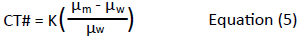
Where μm (obtained during the calibration of the machine) is the measured attenuation of the material in a voxel and K (1000) is the scaling factor set by the manufacturer. Voxels containing materials that attenuate X-rays more than water (e.g. bone, liver, muscle tissue) have positive CT# whereas less attenuating materials (e.g. adipose tissue, lungs) have negative CT#. CT# for a given material (except water and air) will vary with changes in X-ray tube potential as well as across manufacturers [6].
Image noise
Noise is the portion of a signal from an object, that contains no information and it is characterised by a grainy appearance on the image. An image from a CT scanner usually shows CT values fluctuating around a mean value. This random variation (standard deviation) is the image noise. There might be some other deviations present known as structured noise or artefacts. The noise is normally expressed as the normalised standard deviation (SD) of an array CT values at the centre of a single scan of a uniform water equivalent phantom. An array of CT numbers is selected using a region of interest (ROI) with the image diagnostic tool.
In order to make a direct comparison between CT scanners with different contrast scales, a normalised standard deviation (S), also known as % normalised noise (Noise %) is required.
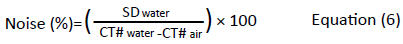
Where; SDwater is the standard deviation of pixel values within a ROI from an image of a uniform medium, whereas CT#water and CT#air are CT values of water and air respectively [7].
Effects of radiation exposure
Many factors determine the biological response to radiation exposure. These factors include variables associated with the system being irradiated and the radiation source. Effects of radiation damage at cellular or molecular level may or may not result in clinically detectable adverse effects. Some effects are quick to appear while some may take decades to appear. Biological effects of radiation are classified into two groups, stochastic and deterministic. Stochastic effects (especially cancer) are considered to be the main health risk from radiation doses less than 100 mGy. Stochastic effects have no threshold dose and the probability of an effect increases with dose, but severity of the effect is not dose related. Deterministic effects such as skin injuries and cataract formation, occur when the radiation exposure is high and once a threshold of exposure has been exceeded. With deterministic effect, the predominant biological effect is cell killing. Appropriate radiation protection mechanisms and occupational exposure dose limits can be put in place to reduce the likelihood of these effects occurring [8].
Aim
The aim of this study was to set-up a protocol for using the CeIT elliptical test phantom to test the performance of Automatic Exposure Control (AEC) systems on the CT scanners in use at Aberdeen Royal Infirmary (ARI). These are the GE Lightspeed, GE Optima 6600 and Siemens Somaton Definition in Radiology and the Philips Brilliance in Radiotherapy treatment planning.
The study focused on the following areas in order to formulate a testing protocol:
Specific aim 1: Understand different AEC systems on different scanners (GE, Siemens and Philips)
Specific aim 2: Evaluate how the image noise varies across the phantom for the three scanners
Specific aim 3: Evaluate the effects of different scouts and different heights on AEC systems of the scanners
Specific aim 4: Formulate a testing protocol to test the performance of AEC systems across scanners
Materials and Methods
The Phantom
The phantom employed was a CeLT Phantom (Figure 1). CeLT Phantom consists of four (4) interlocking and overlapping solid ellipsoids of uniform composition, sized to provide similar attenuation levels as those found across a range of typical patient sizes. Embedded within each ellipsoid are three samples of different materials (contiguous within each section). These materials cover the Hounsfield unit range typically found in patients (+330 HU to -100 HU). There are also two channels which are unfilled so it is also possible to measure air throughout the phantom. Measurement of liquid (water or other material, e.g. radiographic contrast material) is possible if a suitable container is purchased. The phantom was labelled part A-D in the order of increasing size for clarity during the analysis. The weights of each ellipsoid were as follows; A=3.1 kg, B=4.7 kg, C=6.5 kg and D=7.4 kg, with the total weight of the phantom being 33.2 kg. The phantom was centred during the CT acquisition, as in routine CT examination, with the smallest part of the phantom (Part A) going first into the scanner.

Figure 1: CeLT phantom in a CT scanner.
CT Scanners
The phantom was imaged using the three scanners; GE, Siemens and Philips. Since different manufacturers apply AEC systems differently, it was not easy to set common parameters for the three scanners. The scanners operations differed depending on whether it is a 16-slice or 64-slice scanner. Different scanner settings for the three scouts (AP, LAT and PA) for each scanner were as shown in Tables 1 and 2 below.
| Manufacturer | Model | AEC system | Tube current stored in DICOM | kVp | Rotation time (s) | Reconstruction kernel | ||||||||
|---|---|---|---|---|---|---|---|---|---|---|---|---|---|---|
| GE Medical System | Discovery CT750 HD | SmartmA | mA/rotation | 120 | 0.8 | Standard body | ||||||||
| Siemens | SOMATOM Definition AS+ | Care Dose 4D | Effective mAs | 100 | 0.5 | B20f | ||||||||
| Philips | Brilliance Big Bore | Z-DOM ACS & D-DOM | mAs/slice | 120 | 1.453 | Standard body | ||||||||
| Scanner | AEC System | Protocol name | Table position (cm) | Image quality |
|---|---|---|---|---|
| GE | Smart mA | Medium Abdomen Pelvis | 0 | NI=44 Min mA=10 Max mA=400 |
| -10 | ||||
| 10 | ||||
| Siemens | Care Dose 4D | Head Routine | 0 | Effective mAs=261 Quality reference mAs=230 |
| Philips |
Z-DOM | Pelvis/Pelvis | mAs/slice | |
| 0 | 138-694 | |||
| -13 | 56-284 | |||
| 10 | 58-298 | |||
| D-DOM |
Pelvis/Pelvis | mAs/slice | ||
| 0 | 30 | |||
| -13 | 290 | |||
| 10 | 298 |
Table 2: Imaging parameters used to acquire data for all scouts (AP, LAT and PA) Table positions: 0=isocenter, negative values=table below 0 and positive values=table above 0.
The GE and Siemens scanners operated on combined AEC systems (Smart mA and Care Dose 4D) respectively and the Philips scanner operated on the Z-DOM and D-DOM separately as the scanner has no combined AEC system.
Computational implementation
A computer programme, ImageJ, was used to read relevant data from the images obtained from scanning the phantom with each of the scanners. Five ROI of the same area per scanner, with areas ranging from 1089.4 mm2 to 1096.1 mm2 were drawn on the image of the smallest part of the phantom, with numbering of 1 to 5 (drawn in yellow) to represent each ROI. ROI 5 represented the background. It was not easy to maintain the same area of ROI across the scanners, and in some cases within one scanner, when moving across different patient table height, hence a range of the area for the ROI was used. The ROI were drawn about 2 mm from the edge of the smallest image avoiding small circles that appeared on the phantom as they were of different densities from the entire phantom. Measurement of the CT# and corresponding SD values per slice were read from the images using ImageJ (Figure 2).

Figure 2: CT# and corresponding SD per slice from ImageJ.
A macro (Figure 3) was developed on ImageJ to read the desired parameters (kVp, mA, exposure time, slice thickness, amongst others) from the DICOM header. Values obtained from using ImageJ were tabulated and processed to study the effect of AEC on different scanners. The main parameters of interest being the variation of mAs and the image noise across the phantom from different scanners at different SPR.

Figure 3: ImageJ macro presenting data from the DICOM header.
Image quality evaluation
CT# and corresponding SD values from ImageJ were used to study the effects of AEC systems of different scanners on the image noise. Values of measured SD were plotted against slice positions to study how noise varied across the phantom for all scanners. Noise (%) was calculated and compared to average mAs values across the phantom across all scanners. The variation of the CT# and corresponding SD per section of the phantom were respectively presented using the coefficient of variance (CoV). Image slices which showed negative CT#s were excluded from analysis as they either represented beginning or the end of each phantom section or the gap in between phantom sections.
Results
Image noise across the phantom
GE scanner: The standard deviation (showing the noise variation) increased with the phantom, in all ROI (Figures 4a, 4b, 5a and 5b). CeLT phantom is elliptical hence the lateral cross section is bigger than the AP/PA cross section, hence more Xrays were attenuated along the LAT scanning direction as shown in Figure 1a below. ROI 4 at the PA cross section however showed bigger variations compared to other three ROI (Figure 5a and 5b). The reason being that ROI 4 is just above the patient table hence the table also attenuates X-rays leading to AEC system increasing the tube current for enough X-rays to reach the detector to form a good image. The SD increased with the phantom so as to maintain a constant image noise. NB: The sudden decrease and rise in figures below represent negative CT#s at the start or end of each section of the phantom which were excluded from analysis as they represented gaps between phantom sections.

Figure 4: Standard deviation against slice position. ROI 1 and 3 represent the lateral scanning direction, while ROI 2 represents the AP scanning direction.

Figure 5: Standard deviation against slice position. ROI 3 the lateral scanning direction, while ROI 2 and 4 represent the AP and PA scanning directions respectively.
Siemens scanner: The noise variation for the Siemens scanner followed a similar pattern to the GE scanner (increased with the phantom), except for the largest part of the phantom where the noise variation was not consistent within this part of the phantom (Figure 6a, 6b, 7a and 7b).

Figure 6: Standard deviation against slice position. ROI 1 and 3 represent the lateral scouts, while ROI 2 and 4 represent the AP and PA scouts respectively.

Figure 7: Standard deviation against slice position. ROI 1 and 3 represent the lateral scouts, while ROI 2 and 4 represent the AP and PA scouts respectively.
Philips scanner
Z-DOM modulation:The image noise for the Philips scanner on the Z-DOM modulation with the table at the isocenter, followed a similar trend to the GE scanner where the noise was kept almost constant throughout the scanning process (Figures 8a, 8b, 9a and 9b). ROI 4 which is on the side the phantom is in contact with the table also showed bigger values for the SD as more mAs as the table also attenuated some X-rays, which was not the case with the other three ROI.

Figure 8: Standard deviation against slice position for the Z-DOM modulation with the patient table at the isocenter.

Figure 9: Standard deviation against slice position for the Z-DOM modulation with the patient table at the isocenter.
D-DOM: The angular modulation on the other hand presented an increasing pattern in the SD values across the phantom. With this pattern, the image noise remained almost constant within a section of the phantom and jumped to a bigger values as the phantom increased in size (Figures 10a, 10b, 11a and 11b). There was no significant variations in SD values for ROI 1, 2 and 3, while PA scout on ROI 4 showed higher SD values compared to the AP scanning direction (ROI 2).

Figure 10: Standard deviation against slice position for the angular modulation with the patient table at the isocenter.

Figure 11: Standard deviation against slice position for the angular modulation with the patient table at the isocenter.
The variation of the mAs across the phantom
GE scanner: Tube current-time product (mAs) values increased by 5 to 6 times from the smallest part of the phantom to the largest part of the phantom for all the three scouts (Table 3). The scan that used anteroposterior (AP) SPR had small values of the mAs followed by the lateral (LAT), with the posteroanterior (PA) SPR having the largest mAs values at every section of the phantom. The difference is more pronounced in the larger segments of the phantom (Figure 12). Since the radiation dose is proportional to mAs, the results show that the dose increased with the increasing size of the phantom as expected. Hence comparing parts of the patients with similar tissue densities, larger parts of the patients will attenuate X-rays more than more than smaller parts of the patients. More radiation dose is needed as the phantom size increases to compensate for attenuation of X-rays as they pass through different sections of the phantom, and the dose increases as the size increases. The PA scout had highest values of mAs compared to the other two scouts because the patient table also attenuated some X-ray photons. More dose was needed to compensate for the attenuation of X-rays by both the patient table and the phantom before the X-rays could reach the detectors and give a quality image.
| Section | kVp | Area (mm2) | Average mAs | Mean CT#water | SD (HU) | Noise (%) | ||||||||
|---|---|---|---|---|---|---|---|---|---|---|---|---|---|---|
| AP | LAT | PA | AP | LAT | PA | AP | LAT | PA | AP | LAT | PA | |||
| A | 120 | 1096.1 | 21.7 | 23.4 | 31.1 | 19.3 | 19.3 | 19.2 | 18.5 | 17.9 | 15.3 | 1.9 | 1.8 | 1.5 |
| B | 120 | 1096.1 | 40.6 | 46.4 | 56 | 15.5 | 15.5 | 15.4 | 21.6 | 20.7 | 18.1 | 2.2 | 2.1 | 1.8 |
| C | 120 | 1096.1 | 77.1 | 94.4 | 109.3 | 14.5 | 14.5 | 14.5 | 23 | 20.8 | 19.1 | 2.3 | 2.1 | 1.9 |
| D | 120 | 1096.1 | 117.4 | 150.9 | 165.2 | 22 | 21.1 | 21.9 | 26 | 22.4 | 21.5 | 2.6 | 2.3 | 2.2 |
Table 3: Average mAs values and the measured noise (SD) per section of the phantom for different scouts with the patient position at the iscocenter.

Figure 12: Shows variation of mAs across the phantom for the GE scanner.
Table 4 below show no consistent pattern in the attenuation (CT#) when comparing the four sections of the phantom. The CT numbers’ coefficient of variation (CoV), found by SD ÷ mean, across the phantom was as follows; 11.2%, 7.4%, 7.5% and 35.8% for parts A, B, C and D respectively. The expectation was a consistent attenuation pattern increasing from the smallest to the largest part of the phantom since the phantom is made from the same material with the only difference being the increase in size from part A to part B. However the coefficient of variance (CoV) of the noise across the phantom (sections A to D) was consistent with values of 16.5%, 16.5%, 16.6% and 16.7% respectively.
| Phantom Section | Mean CT#water | SD | Noise (%) | CoV (%) | |
|---|---|---|---|---|---|
| CT# | Noise (%) | ||||
| A | 19.3 | 18.5 | 1.9 | 11.2 | 16.5 |
| B | 15.5 | 21.6 | 2.2 | 7.4 | 16.5 |
| C | 14.5 | 23 | 2.3 | 7.5 | 16.6 |
| D | 22 | 26 | 2.6 | 35.8 | 16.7 |
Table 4: CoV of CT# and noise (%) for the GE scanner-AP.
Siemens: The noise (%) increased with increasing mAs values (AP SPR) across the phantom from part A to part D. The mAs values increased 3 times from the smallest to the largest part of the phantom (Table 5). The variation of the mAs per section of the phantom was not consistent. The tube current however saturated (became constant) at the largest (most attenuating) part of the phantom (Figure 13). The CoV of CT# and SD increased with the phantom, with values of 4.7% to 9.5% and 9.2% to 10.4% for the CT# and SD respectively.
| Phantom Section | kVp | ROI area (mm2) | mAs | Mean CT#water | SD | Noise (%) | CoV | |
|---|---|---|---|---|---|---|---|---|
| CT# | Noise | |||||||
| A | 100 | 1089.4 | 117.6 | 11.7 | 8.3 | 0.9 | 4.7 | 9.2 |
| B | 100 | 1089.4 | 162.9 | 8.4 | 10.3 | 1.1 | 6.9 | 9.6 |
| C | 100 | 1089.4 | 261 | 8.2 | 12.3 | 1.3 | 8.4 | 9.9 |
| D | 100 | 1089.4 | 323.5 | 8.8 | 13.6 | 1.4 | 9.5 | 10.4 |
Table 5: Average mAs values with corresponding CT#, SD and noise (%) for the Siemens scanner.

Figure 13: Shows variation of mAs across the phantom for the Siemens scanner.
Philips: The mAs increased with the phantom for the Z-DOM modulation (Figure 14), with an increase of 5 times from part A to part B of the phantom. The mAs was kept almost constant within each section of the phantom. The angular modulation mAs decreased linearly with the increasing size of the phantom (Figure 14). The linear decrease was 12.2% with average mAs values of 245.8 mAs at the smallest part of the phantom and 215.7 mAs for the largest part of the phantom.

Figure 14: Shows variation of mAs across the phantom for the Philips scanner.
The % noise for the Z-DOM modulation was almost consistent (0.8% to 1.0%) with increasing mAs values across the phantom (Part A to D), as shown in Table 6 below. The angular modulation on the other hand had significant increase in the % noise (0.4% to 1.2%) from the smallest part (A) to the largest part (B), with the corresponding mAs values decreasing from part A to D (245.8 mAs to 215.7 mAs). For the Z-DOM, the CoV for the CT numbers (Table 7) decreased from part A to part D except in part C where the CoV was the highest (10.2%). The CoV values for the CT# (angular modulation) followed a similar trend as in the Z-DOM modulation, with part C of the phantom having the highest value of 9.7%. The CoV for the SD values followed no consistent pattern, with values ranging between 4.9% to 6.7% for the Z-DOM and 3.8% to 5.1% for the angular modulation.
| Phantom Section | kVp | ROI area (mm2) | mAs | Mean CT# | SD | Noise (%) | CoV | |
|---|---|---|---|---|---|---|---|---|
| CT# | SD | |||||||
| A | 120 | 1093.2 | 61.8 | 13.2 | 7.5 | 0.8 | 9.1 | 6.2 |
| B | 120 | 1093.2 | 103.8 | 10.3 | 8.6 | 0.9 | 7.9 | 6.7 |
| C | 120 | 1093.2 | 178.9 | 11.6 | 9.5 | 1 | 10.2 | 6.3 |
| D | 120 | 1093.2 | 282.4 | 11.8 | 9.5 | 1 | 4.7 | 4.9 |
Table 6: Relationship between mAs and noise (%) for the Z-DOM modulation.
| Phantom Section | kVp | ROI area (mm2) | mAs | Mean CT#water | SD | Noise (%) | CoV | |
|---|---|---|---|---|---|---|---|---|
| CT# | SD | |||||||
| A | 120 | 1093.2 | 245.8 | 13.3 | 3.7 | 0.4 | 8.9 | 4.4 |
| B | 120 | 1093.2 | 236.3 | 10.4 | 5.6 | 0.6 | 7.7 | 5.1 |
| C | 120 | 1093.2 | 227.4 | 11.9 | 8.4 | 0.9 | 9.7 | 3.8 |
| D | 120 | 1093.2 | 215.7 | 12.2 | 11.4 | 1.2 | 4.5 | 4.6 |
Table 7: Relationship between mAs and noise (%) for the angular modulation.
Effects of different scouts and different heights on AEC systems of the scanners
Different table heights using the AP scout
GE scanner: Lower values of mAs were recorded at the table height 10 cm below the isocenter (Figure 15). The AEC system views the phantom to be further, therefore smaller from the X-ray tube thereby delivering lower mAs. When the patient table was 10 cm above the isocenter, higher values of mAs were recorded. The table height above the isocenter takes the phantom closer to the X-ray tube, hence the AEC system views the phantom as larger (magnified), where higher values of mAs will be needed to compensate for X-rays attenuation to obtain a good image, thereby delivering a higher dose.

Figure 15: mAs across the phantom at different patient table heights for the GE scanner.
Philips scanner: The variation of the mAs at different table heights followed a similar pattern as with the GE for the Z-DOM modulation, with higher values of mAs obtained at each phantom section for the table height of 10 cm above the isocenter (Figure 16a). The table height of -13 cm below the isocenter presented lower values of mAs. The angular modulation did not show significant difference in variations of the mAs at different table positions (Figure 16b).

Figure 16: mAs across the phantom at different patient table heights for the Philips scanner for (a) the Z-DOM modulation and (b) angular modulation.
Comparison of AEC performance and corresponding noise (%) across the phantom on the three scanners
AEC testing protocol: The following steps should be followed when testing the performance of AEC systems in CT scanners using CeLT phantom.
Ensure correct positioning of the phantom on the table with the smallest part first into the gantry
Set scanning parameters as stipulated in Tables 1 and 2 for each scanner
Start imaging the phantom
Change the table position to image at different positions above and below the isocenter
Compare results to the ones in Tables 3-8
Accept the test if results fall within 10% of the ones in Tables 3-8
Check scanning parameters once again if results fall outside 10% range of the ones in Tables 2 and 6
This testing protocol is to ensure proper CT scanner operation as is directly related to the quality of patient care. The 10% tolerance was arbitrary chosen and when test results fall way beyond this limit, the manufacturers tolerance limits should be used.
Discussion
AEC systems have been broadly accepted in clinical practice as an effective method for adapting dose to patient size, anatomy of the scanned region and the direction of scanning. Challenges posed by different manufacturers’ application of AEC systems require CT scanner users to understand algorithms to be used for each specific scan to minimise patient over/under exposure to radiation without compromising image quality [9]. Several studies have shown a significant patient dose reduction without compromising image quality when AEC systems are used in CT [3,5,10]. There are several aspects to consider with the use of AEC systems in CT scanning and the localiser (SPR) being one fundamental aspect as it provides information on the attenuation of the patient [11].
AEC systems on different scanners (GE, Siemens and Philips)
The results show that AEC systems of all the three scanners adjusted the mAs with relative to the size of the phantom, with higher mAs values for bigger parts of the phantom and smaller mAs values for the small part of the phantom, except for the Philips angular modulation where mAs decreased with increasing size of the phantom (Table 8).
| Phantom section | Average mAs | Noise (%) | ||||||
|---|---|---|---|---|---|---|---|---|
| GE | Siemens | Philips | GE | Siemens | Philips | |||
| Z-DOM | Angular | Z-DOM | Angular | |||||
| A | 21.7 | 117.6 | 61.8 | 245.8 | 1.9 | 0.9 | 0.8 | 0.4 |
| B | 40.6 | 162.9 | 103.8 | 236.3 | 2.2 | 1.1 | 0.9 | 0.6 |
| C | 77.1 | 261 | 178.9 | 227.4 | 2.3 | 1.3 | 1 | 0.9 |
| D | 117.4 | 323.5 | 282.4 | 215.7 | 2.6 | 1.4 | 1 | 1.2 |
Table 8: Comparison of the variation of mAs and corresponding noise (%) for all scanners for the AP SPR.
The GE scanner operates on the principle of keeping a constant image noise across all patient. A noise index (NI) chart could be used for scanners using the constant image noise approach, where the mA modulation is done manually for patients of different sizes, with higher noise indices for large patients and lower noise indices for smaller patients [9].
The Siemens Care Dose 4D operates on the principle that different patient sizes require different levels of noise to maintain adequate image quality. This is achieved by assessment of the size of the scanned cross section and adjusting the mA relative to the reference mAs. The Siemens scanner showed higher mAs values for large sizes and smaller mAs values for smaller sizes.
The Siemens and the Philips scanners mA values are determined by the scanners and depend on settings that increase the noise level with patient size, while the GE scanner minimum and maximum mA values are selected and the mA is modulated within the range of selected image noise levels. mA values used in the GE and Philips scanners are based on SPRs attenuation levels, while the Siemens scanner uses the SPR to estimate the mA range, and the mA are adjusted based on real time measurements of attenuation during the scan as shown in Table 8.
How image noise varies across the phantom for the three scanners
Results from this study show an increase in noise (%) with increasing size of the phantom for the three scanners (Table 8). The increase in noise (%) was a result of more attenuation of Xrays by larger parts of the phantom.
Effects of different scouts and different heights on AEC systems of the scanners
The PA scout resulted in higher mAs values across the phantom for the GE scanner and this shows the importance of choosing the appropriate SPR for dose matching to the patient examination. Different SPR were not examined with the other two canners (Siemens and Philips).
Different table heights (Off-centering)
Modern CT scanners use beam-shaping (bowtie) filters to reduce patient dose and improve image uniformity. Horizontal off-centering could lead to increase in radiation dose and excessive radiation dose to radiosensitive superficial structures such as breasts, thyroid and gonads. Horizontal off-centering could also result in poor image quality as the most attenuating part of the scanned area (center) receives few X-rays hence noisier images will be obtained. Vertical off-centering (in AP/PA scout scanning) could either diminish or magnify the scanned region leading to the AEC system adapting the mA to wrong values which will in turn result in either noisier images (for diminished regions) or unnecessary increase in dose (for magnified regions). Vertical off-centering in both cases of the GE and the Philips scanners resulted in higher mAs values for table heights above the isocentre and lower mAs values for table positions below the isocenter. This relationship was not studied with the Siemens scanner.
Conclusion
AEC systems that provides combined modulation and in which acceptable image noise levels are varied according patient size, region scanned, and diagnostic task have shown to provide significant levels of dose reduction [3,5,10,11]. The results of this study show that the dose and consequently image noise is dependent on the anatomy and size of the scanned region, for which a specific examination protocol is examined. The Philips D-Dose should be used with care as it did not regulate dose based on attenuation of the phantom and it delivered high dose at smaller parts of the phantom. This could result in high doses to children or small patients than necessary. Several aspects of AEC systems should be considered when optimising CT radiation dose. These aspects include patient positioning and centering, the projection angle of the localiser, protocol selection, and the use of protective devices. Evaluation of AEC systems is an important aspect of the QC of CT scanners in monitoring patient dose as well as obtaining useful quality images for patient management and care. CeLT phantom was useful in studying how AEC on different scanners regulate dose and corresponding noise to provide a clinically useable image. The results obtained were useful in formulating a testing protocol to be used in monitoring the performance of CT scanners in regulating patient dose and providing clinically useful images.
References
- McCollough C, Branham T, Herlihy V, Bhargavan M, Robbins L, et al. ( 2011) Diagnostic reference levels from the ACR CT Accreditation Program. J Ame Radiology 8: 795-803.
- Foley SJ, Mcentee MF, Rainford L A (2012) Establishment of CT Diagnostic Reference Levels in Ireland. The British J Radiology 85: 1390-1397.
- Wood TJ, Moore CS, Stephens A, Saunderson JR, Beavis AW (2015) A practical method to standardise and optimise the Philips DoseRight 2.0 CT Automatic exposure control System. J Radio Prot 38: 495-506.
- Solomon JB, Li X, Samei E (2013) Relating Noise to Image Quality Indicators in CT examinations with Tube Current Modulation. AJR 200: 592-600.
- Merzan D, Nowik P, Poludniowski G, Bujila R (2017) Evaluating the impact of scan setting on automatic tube current modulation in CT using a Novel Phantom. British J Radiology 90: 20160308.
- Mahesh M (2002) The AAPM/RSNA Physics tutorial for residents. Search for isotropic resolution in CT from conventional through multiple-row detector. Radiographics 22: 949 -962.
- Edyvean S, Lewis M A, Jones A P (2003) Measurement of the performance characteristics of diagnostic X-ray systems used in medicine. Report no.32 Part III. Computed Tomography X-ray Scanners. 2nd Edn. Institute of Physics and Engineering in Medicine: York: 12-13.
- Mettler FA (2012) Medical effects and risks of exposure to ionising radiation. J Radio Protec 32: N9 -N13.
- Kelly AM, Cronin P (2015) Practical approaches to quality improvement for radiologists. RadioGraphics 35: 1630-1642.
- Soderberg M (2016) Overview, practical tips and potential pitfalls of using automatic exposure control in CT: Siemens Care Cose 4D. Radiation Protec Dosimetry 169: 84-91.
- Favazza CP, Yu L, Leng S, Kofler JM, McCollough CH (2015) Automatic exposure control systems designed to maintain constant image noise: Effects on computed tomography dose and noise relative to clinically accepted technique charts. Journal of Computer Assisted Tomography 39: 437-442.

Open Access Journals
- Aquaculture & Veterinary Science
- Chemistry & Chemical Sciences
- Clinical Sciences
- Engineering
- General Science
- Genetics & Molecular Biology
- Health Care & Nursing
- Immunology & Microbiology
- Materials Science
- Mathematics & Physics
- Medical Sciences
- Neurology & Psychiatry
- Oncology & Cancer Science
- Pharmaceutical Sciences